| Uwe B. Meding | » Get the PDF | » Get the Source |
Principal Components Analysis (PCA) is a great tool of modern data analysis. It follows two related goals: It tries to find a good data representation by only focusing on the features part. A side effect of this focus is that it also reduces the redundancy in the data.
Another way to interpret PCA is that there is some variable which accounts for a percentage of the variation in your data. What this hidden variable is is unclear. However, given that your primary eigenvector accounts for say 45% of all the variation in your sample implies that the effect of this number one hidden variable is quite large.
What is this hidden factor? That answer depends very much on your data. Nearly every measurement in the sample data has a correlation to it. Maybe
it’s temperature changes, or day and night cycles, or some other reason. You cannot determine what the hidden variable is. However, you can determine
that it exists.
Principal Components Analysis
Formally, PCA tries to find the linear combination within a set of variables for which the vector of covariances is of greatest length. This is done through using eigenvectors, specifically by calculating the covariance matrix among the variables. The largest eigenvalue and the corresponding eigenvector represent the direction of the highest variation.
The PCA can be used on any signal that comprises a set of correlated data sequences. For example, in image processing a film sequence comprises a set of correlated images. In energy usage analysis, which is expressed as a waveform that represents a correlated set of individual components.
PCA is a way of identifying patterns in data, and expressing the data in such a way as to highlight their similarities and differences. Since patterns in data can be hard to find in data of high dimension, where the luxury of graphical representation is not available, PCA is a powerful tool for analyzing data. The other main advantage of PCA is that once you have found these patterns in the data, and you compress the data, ie. by reducing the number of dimensions, without much loss of information. This technique used a lot in image compression.
- PCA completely decorrelates the original signal. Formally speaking, the transform coefficients are statistically independent for a Gaussian signal
- PCA optimizes the repacking of the signal energy, such that most of the signal energy is contained in the fewest transforms coefficients.
- It minimizes the total entropy of the signal
- For any amount of compression the mean squared error (MSE) in the reconstruction is minimized.
Given these abilities, PCA should be in widespread use. However, there are several drawbacks to PCA, the greatest being the computational overhead required to generate the transform vectors. The transform vectors for the PCA are the eigenvectors of the auto-covariance matrix formed from the data set.
The following recipe generates the principal component vectors for a signal
1.1 Method
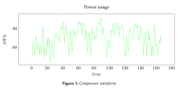
- Step 1: Get some data
- In Figure 1, we are using measured power usage data set for a compressor. We could reduce it to 2 dimensions, however, this would also limit our analysis to rough measures. Instead we will be using Toeplitz matrices to represent the waveform, and thereby create a lot more dimensions to analyze.
- Step 2: Construct an average signal
- For PCA to work properly, you have to subtract the mean from each of the data
dimensions.
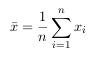 The mean subtracted is the average across each dimension. So, all the x values have
x̅ (the mean of the x values of all the data points) subtracted, and all the y values have y̅ subtracted from them. This produces a data set whose mean is zero. - Step 3: Calculate the covariance matrix
- Since the data is n dimensional (the Toeplitz matrix representation provides a dimension for each point), the covariance matrix will be n × n.

For example, the covariance matrix for an 3 dimensional data set, using the usual
dimensions x, y and z. Then, the covariance matrix has 3 rows and 3 columns, and
the values are this:
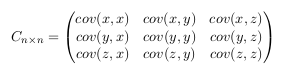
This matrix has some interesting properties: Down the main diagonal, the covariance
values are between one of the dimensions and itself. These are the variances for
that dimension. The other point is that since cov(a, b) = cov(b, a) , the matrix is
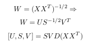
symmetrical about the main diagonal. - Step 4: Calculate the eigenvectors and eigenvalues of the covariance matrix
- Covariance matrices are positive definite, therefore they are symmetric and will
have orthogonal eigenvectors and real eigenvalues. The covariance matrices are
factorizable using:

Where U has eigenvectors of A in its columns and Λ = diag(λi), where λi are the
eigenvalues of A. There are various ways to find a solution for the eigenvectors U
and and the eigenvalues Λ of Cov(X), here we are using singular value decomposition
(SVD).
All the eigenvectors are normalized to have unit energy, to give an orthogonal transform. The corresponding eigenvalues for these vectors show the variance distribution of the ensemble within this transform domain. This indicates how effective the repacking of the signal energy is likely to be with these vectors. This is very important for PCA, but luckily, most maths packages, when asked for eigenvectors, will
give you unit eigenvectors.So, by this process of taking the eigenvectors of the covariance matrix, we have been
able to extract lines that characterize the data. - Step 5: Determine the principle components
- The principle components are determined by using the principle factors V and relating back to the original data
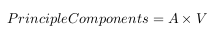
This is where the notion of data compression and reduced dimensionality comes into
it. The eigenvector with the highest eigenvalue is the principle component of the data
set. In our example, the eigenvector with the largest eigenvalue was the one that
pointed down the middle of the data. It is the most significant relationship between
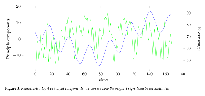
the data dimensions. Figure 2 show the largest 4 principle components.The eigenvalues, see Figure 4, give a measure of how the energy in the transform is
distributed, and so indicate how well the energy of the signal will be redistributed
in the transform. The first four eigenvectors of this transform represent about 80% of
the transform energy, which means that discarding higher order vectors would, on
average, lead to a decreasing error.

1.2 Interpretation
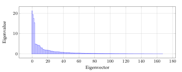
Figure 5 is related to the eigenvalues, and reflects the quality of the projection from the
N-dimensional initial table (N = 168 in this example) to a lower number of dimensions.
In this example, we can see that the first 6 eigenvalues about 50% of the total variability.
This means that if we represent the data on only one axis, we will still be able to see 50%
of the total variability of the data.
Each eigenvalue corresponds to a factor, and each factor to a one dimension. A factor
is a linear combination of the initial variables, and all the factors are uncorrelated. The
eigenvalues and the corresponding factors are sorted by descending order of how much
of the initial variability they represent (converted to %).
Ideally, the first two or three eigenvalues will correspond to a high % of the variance,
ensuring us that the maps based on the first two or three factors are a good quality projection
of the initial multi-dimensional table. In this example, the first six factors allow us to
represent 50% of the initial variability of the data. This is a decent result, but we will have
to be careful when we interpret the maps as some information might be hidden in the next
factors. We probably will need 25-30 factors to represent more than 80% of the variability.
We can see that the number of “useful” dimensions has been automatically detected.
Figure 6 shows the correlation circle. It shows a projection of the initial variables in the
factors space.
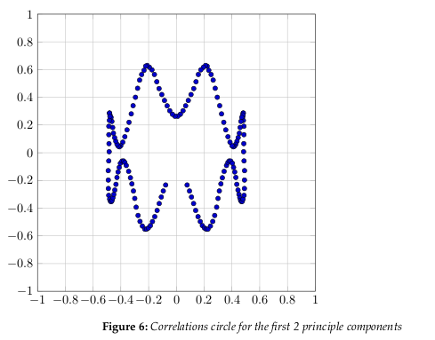
In general, when two variables are far from the center
- If they are close to each other, they are significantly positively correlated (r ≈ 1)
- If they are orthogonal, they are not correlated (r ≈ 0)
- If they are on the opposite side of the center, then they are significantly negatively correlated (r ≈ −1)
When the variables are close to the center, it means that some information is carried on
other axes, and that any interpretation might be hazardous.
The correlation circle is useful in interpreting the meaning of the axes. In our example,
we can see that certain areas correlate more than others. Overall, it is apparent the correlation is somewhat weak, as we have already determined by the number of factors we need
to represent 80% of the data.
References
- Alexander Basilevsky, Applied Matrix Algebra in the Statistical Sciences. Dover Publications, 1983 Edition, 2005.
- Herve Abdi1 and Lynne J. Williams , Principal component analysis, John Wiley & Sons, WIREs Computational Statistics, Volume 2, July/Aug 2010.
- Jon Shlens, A tutorial on Principal Component Analysis, UCSD, March 2003.
- Wikipedia, Toeplitz matrix, http://en.wikipedia.org/wiki/Toeplitz_matrix


Leave a Reply
You must be logged in to post a comment.